Tip of the Week: Freeze Microsoft Excel Panes

In the right hands, Microsoft Excel can be an incredibly potent data management tool. Unfortunately, scrolling down will leave your headers out of sight unless you take steps to freeze them in place. Let’s discuss how you can do this and be more productive with this tool.

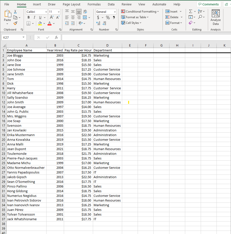
To showcase how to do this, let’s use some fake data detailing departments within your business, their employees, their date of hire, and their current rate of pay.

Scrolling down this long list would be irritating without knowing which column is which. For something like this, it’s not terribly inconvenient, but for more complicated spreadsheets, it will be a necessity. Excel has functionality to keep certain data on-screen at all times.

Time to Freeze Your Panes

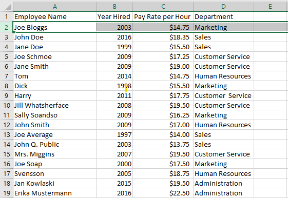
To freeze panes in Excel, you just have to tell it what data you want to remain visible while you scroll. It’s remarkably easy to do. First, select the row immediately below or the column immediately to the right of the data you want to be frozen. For the purposes of this example, you’d want to keep Row 1 in sight, so we would use Row 2 for the setting.

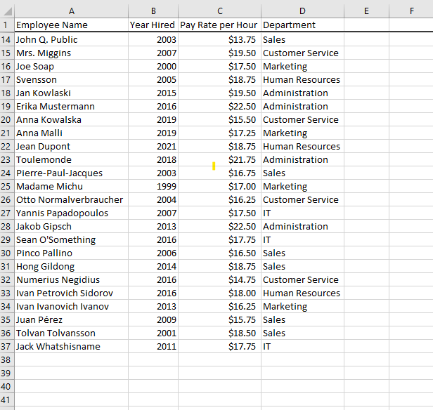
Now that the column or row is selected, you’ll use the View tab to find the Freeze Panes option. You should then see three options: Freeze Panes, Freeze Top Row, or Freeze First Column. For our example, we would want to use Freeze Panes (but in this context, Freeze Top Row would also be acceptable). Now you should see that, when you scroll down, the top row will remain in place.

It’s that easy! Now you can keep important data showcased at the top or left while you go about your work. If you want to know more about how to make the most of your business technology, be sure to contact us at (954) 739-4700.